Maximum Likelihood Estimaton on Pixel Classification

Introduction

The task in computer vision is usually connected with identifying different object, segmenting regions of interest and classifying them.

Remote sensing is the process of acquisition of data, usually about he Earth surface, through processes that do not involve physical contact. Today it is usually done through aerial sensor technologies that detect and classify objects on the ground. They are split into active remote sensing (when energy is transmitted into the environment) and passive.

In our case, there is data obtained from both methods.
• Passive: RGB camera; Near Infrared camera.
• Active: LiDAR - recording of the first and the last echo.

So let’s assume we have the following RGB image along side a near infrared image and LiDAR data (first echo - fe and last echo - le):

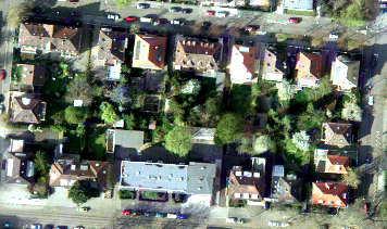
RGB image of the area to classify

And the requirement is to extract the areas that are buildings, vegetation, ground or cars.
From a statistical perspective one way to achieve this would be to build a model of the pixel for each of the above classes.

It can be assumed that for instance the ground pixel values will be forming a Gaussian distribution.
So the probability density function will look like:

$$p(x|\omega_i)=\frac{1}{{(2\pi)}^{n/2}\sqrt{|\Sigma_i|}}, e^{-\frac{1}{2}[(x - \mu_i)^T\Sigma_i^{-1}(x - \mu_i)]}$$

where $\mu_i$ is the mean vector of our data samples for a given class and $\Sigma_i$ is the covariance matrix and n - dimensionality of our vector.

In our case, the pixel is actually a 6 dimensional vector consisting of the [R, G, B, nIR, fe, le]. In order to build our model we require samples for each class. It is usually assumed to have 10 times the dimensionality of your vector as number of samples, but in limiting cases that can go down to 3-4.
To obtain those, one would have to manually select pixels corresponding to each class. Luckily, we have a ground truth image with pre-labelled pixels. For good measure, 50 data points will be sampled for each class.

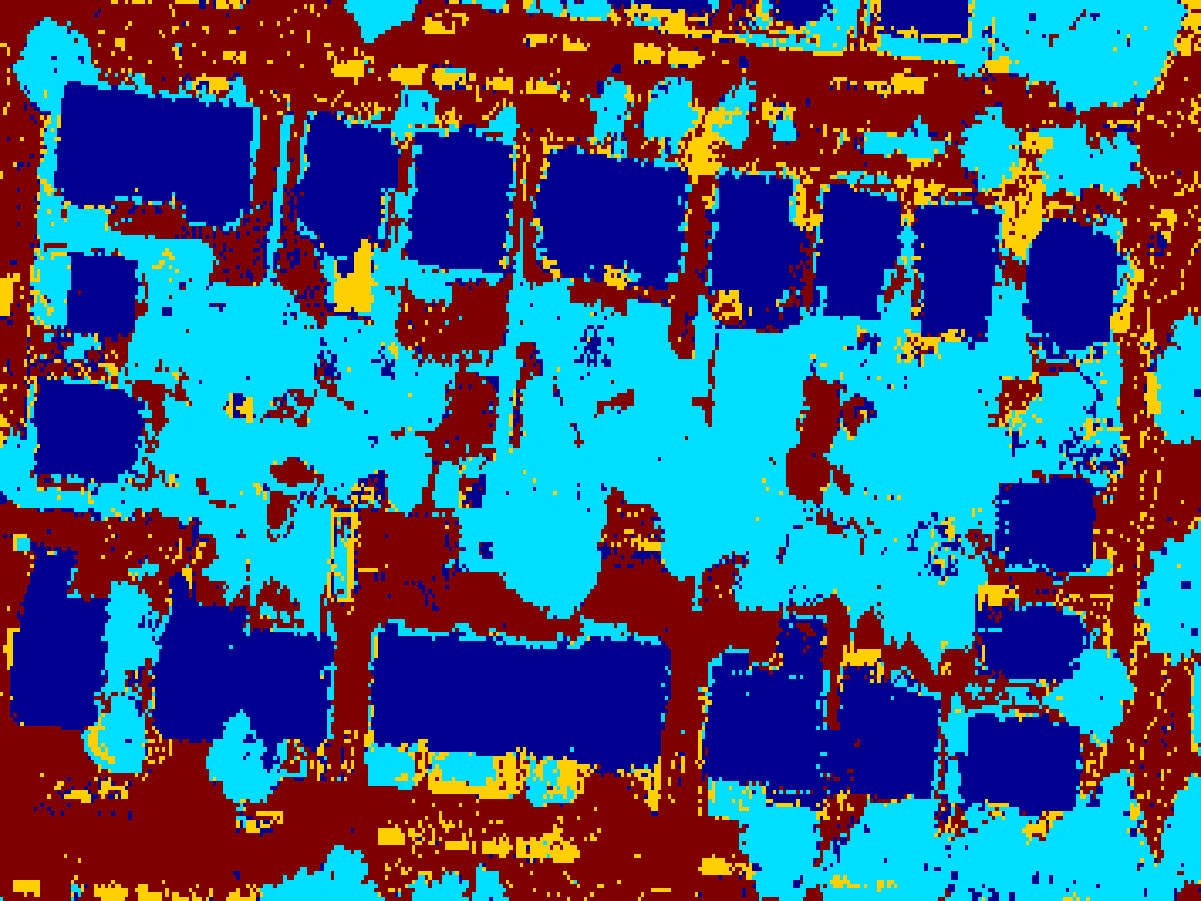
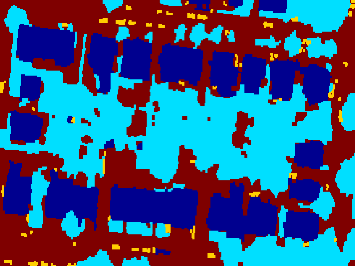
Ground Truth image. Dark Blue - Buildings; Light Blue - Vegetation; Yellow - Cars; Red - Ground.

Obtaining samples

The samples obtained need to be selected at random in order to best represent the data. Thus, one can select all pixels corresponding to a single class and choose at random 50 of those. 

For instance a crude version of this in MATLAB will look like: (This needs checking that you are not selecting a pixel twice, that there are enough pixels of that kind, etc):

N = 50; buildings = zeros(0, 6);  
while (size(buildings, 1) < N)  
    x = randi(size(groundtruth, 1), 1);  
    y = randi(size(groundtruth, 2), 1);  
    if (groundtruth(x, y) == 1)  
        buildings(end+1,:)= [b(x, y) g(x, y) r(x, y) nir(x, y) fe(x, y) le(x, y)]';  
    end  
end

Generating model

In order to generate the model for each of the classes, you need to find the mean and the covariance!

This is easy in MATLAB:

s_mean = mean(sample)';  
s_cov = cov(sample)';

Or the corresponding functions in OpenCV - calcCovarMatrix(…).

This needs to be done for each of the classes.

Applying the models

Once we have the models defining how a building, a car, a tree or the ground looks like, we need to apply those to the input data.

This can be accomplished by going over the image and calculating the probability, using the above equation. First we can precompute the scaling/normalization factor and then the exponential part for each pixel.

%Calculate the normalization factor  
norm = 1.0 / (power((2*pi), size(cov, 1)/2) * sqrt(det(cov)));  
% For each pixel, calculate the probability of this model  
for x = 1: size(image, 1)  
    for y = 1: size(image, 2)  
        % Generate current sample  
         X = double([b(x, y) g(x, y) r(x, y) nir(x, y) fe(x, y) le(x, y)]');  
        % Calculate exp part of the probability  
        expo = exp(-0.5 * (X - mean).' * inv(cov) * (X - mean));  
        image(x, y) = norm * expo;  
    end  
end  
end

 If we run that for the 4 models we have stated above, the following results can be obtained:

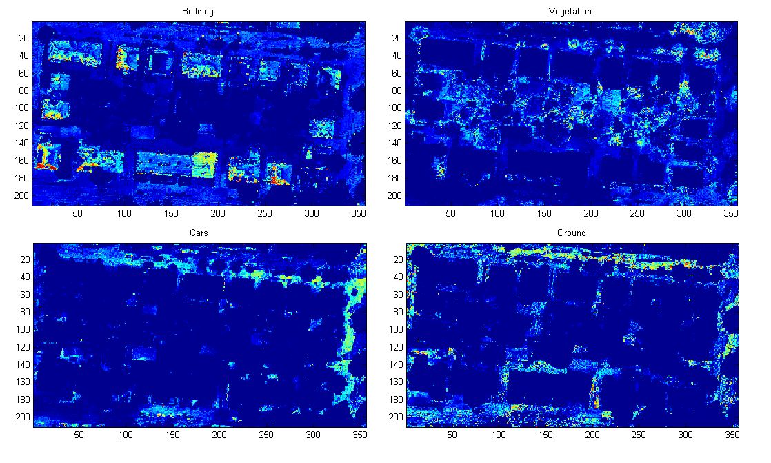
Probabilities for  each of the classes $(b, v, c, g)$.

The next step of applying the algorithm is to actually see which of the classes gives a bigger (maximum) likelihood for each particular area. Then this class will be assigned to that pixel.
In MATLAB a possible solution will be:

function [classified] = merge_classes_mle(b, v, c, g)  
classified = zeros(size(b));  
for x = 1: size(classified, 1)  
    for y = 1: size(classified, 2)  
        A = [b(x,y) v(x, y) c(x, y) g(x, y)];  
        i = find(A==max(A), 1);  
        classified(x, y) = i;  
    end  
end  
end

A combination of those ‘heatmaps’ will be similar to this (different initial conditions will generate a slightly different model resulting in a slightly different final classification).

Estimating error

A simple way to estimate the performance of the classification algorithm is to calculate the confusion matrix. This will give us the number of cases in which an object was misclassified.

Using the ground truth as a model, the following data was calculated:

	Estimated
Ground Truth	B	V	C	G
B	0.7806	0.065	0.0576	0.0968
V	0.0333	0.8701	0.0289	0.0678
C	0.0443	0.0443	0.7041	0.2072
G	0.0546	0.1338	0.073	0.7386

This resulted in an accuracy of 79%.

Applying expert knowledge

As humans, we know a great deal about the world we live in. That information can be used in order to add some “sense” to the algorithm. If we look at the above image, we’ll see that there are a lot of single pixel classification of the class car. We know that it is impossible, thus, those can be removed and substituted with the second best approximation. Also, some of the “cars” are spanning for over 50 pixels and create a non convex shape. We can assume with reasonable certainty that these are false positives as well. 

If we extract the car class and apply the above outlined knowledge, we can get the following result.

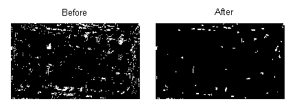
Filtering the car class with expert knowledge.

This looks much better!

Let’s consider the data again, we can extract similar rules for the other classes as well - vegetation, buildings contours are smooth and have a minimum size, don’t exhibit other small instances of classes in them - e.g. small holes. These can be fixed by applied a series of morphological operators. The closing operator, which is a sequence of dilation and erosion, will fill in small gaps in the binary image. Opening at the other hand, will remove small speckles and smooth out the overall shape of the contour.

By applying all the rules, we come to this final classification.

We can see a bigger similarity to the ground truth data. But what does the accuracy and confusion matrix tell us?

If we recalculate it, we get

	Estimated
Ground Truth	B	V	C	G
B	0.7878	0.0551	0.0101	0.147
V	0.0064	0.9175	0.0041	0.072
C	0.0398	0.0986	0.4905	0.371
G	0.0268	0.1328	0.0124	0.8279

And a resulting accuracy of 84%!

As you can see, such a simple method of maximum likelihood estimation, combined with some expert knowledge of the domain resulted in great classification accuracy!

This can be applied to other domain with more classes, or just a single class - e.g. skin detection and works fast enough to be applied in real time.