If you are interested in just seeing the final result, scroll down.

Bokeh and Holoviews are an amazing set of libraries to help us visualize data in an intuitive and interactive way.

Setup

Bokeh code

We’ll assume some familiarity with the Bokeh library, and we’ll discuss more in length the ways to create the plots in the next parts. For now, you can checkout their example page.

You can find the full code for this demo in the bokeh_html_hover.py gist.

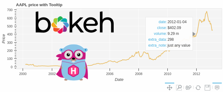
We want to plot the market price of AAPL stock and have the ability to hover over the plot and receive more information about a particular data point. The more important parts are as follows:

# Load the data
source = ColumnDataSource(
    data={
        "date": datetime(AAPL["date"][::10]),
        "adj close": AAPL["adj_close"][::10],
        "volume": AAPL["volume"][::10],
        "extra_data": list(range(len(AAPL["volume"][::10]))),
    }
)

# Create the figure storing the plot
p = figure(
    plot_height=250,
    x_axis_type="datetime",
    tools="pan,wheel_zoom,box_zoom,reset,save",
    toolbar_location="below",
    title="AAPL price with Tooltip",
    sizing_mode="scale_width",
    output_backend="svg",
)
# Additional things to tune
p.toolbar.logo = None
p.background_fill_color = "#f5f5f5"
p.grid.grid_line_color = "white"
p.xaxis.axis_label = "Date"
p.yaxis.axis_label = "Price"
p.axis.axis_line_color = None

# Plot the actual data
p.line(x="date", y="adj close", line_width=2, color="#ebbd5b", source=source)

# The magic to make a hover tooltip showing the data we want
p.add_tools(
    HoverTool(
        tooltips=[
            # use @{ } for field names with spaces
            ("date", "@date{%F}"),
            ("close", "$@{adj close}{%0.2f}"),
            ("volume", "@volume{0.00 a}"),
            ("extra_data", "@extra_data"),
            ("extra_note", "just any value"),
        ],
        formatters={
            "@date": "datetime",  # use 'datetime' formatter for 'date' field
            "@{adj close}": "printf",  # use 'printf' formatter for 'adj close'
            # use default 'numeral' formatter for other fields
        },
        # display a tooltip whenever the cursor is vertically 
        # in line with a glyph
        mode="vline",
    )
)

To pre-fetch the data needed, you can run

python -c "import bokeh; bokeh.sampledata.download()"

Save the plots as JSON files like shown here.

filename = Path(__file__).stem + ".json"
with open(filename, "w") as json_file:
    div_id = "example_plot_with_hover"
    json.dump(json_item(p, div_id), json_file)

In order to test the plot, you can also show() the figure, which will open a browser window locally. This is also useful for debugging, tweaking, visualizing your other projects and especially useful if you’re developing within a e.g. Docker container.

Now that we have the plot we like, let’s see how to embed it into your web-page (in our case - a hugo markdown page).

Pro tip: You can also work directly with the resulting html file and import it as necessary, but I find it lacks the modifiability that comes with storing the data in a data format.

Shortcode

In Hugo, we can create a shortcode that you can think of as an advanced markdown command. It will make the repeating process easier when we are adding multiple plots across our pages.

Now that we have the JSON file, let’s put it into a resource folder and create the shortcode (bokeh.html).

Use the following shortcode (from the discussion here) to load the plot:

{{ $item := $.Page.Resources.GetMatch (.Get 0)}}
<div id="{{ .Get 0 }}">
  <script charset="utf-8" type="text/javascript">
    var xmlhttp = new XMLHttpRequest();
    xmlhttp.onreadystatechange = function() {
      if (this.readyState == 4 && this.status == 200) {
        var item = JSON.parse(this.responseText);
        Bokeh.embed.embed_item(item, "{{ .Get 0 }}");
      }
    };
    xmlhttp.open("GET", "{{ $item.RelPermalink }}", true);
    xmlhttp.send(); 
  </script>
</div>

Place it in the project, bearing in mind the Shortcode Template lookup order

* /layouts/shortcodes/<SHORTCODE>.html
* /themes/<THEME>/layouts/shortcodes/<SHORTCODE>.html

Bokeh JS

We are nearly there. Additionally, we need to load the Bokeh js libraries in the blog post before using the shortcode. We can include them automatically with each post, but we don’t want our page to load unnecessary scripts. You can lookup the latest version from here and in my case they are as follows:

<script type="text/javascript" src="https://cdn.bokeh.org/bokeh/release/bokeh-2.0.1.min.js" ></script>
<script type="text/javascript" src="https://cdn.bokeh.org/bokeh/release/bokeh-widgets-2.0.1.min.js" ></script>
<script type="text/javascript" src="https://cdn.bokeh.org/bokeh/release/bokeh-tables-2.0.1.min.js" ></script>
<script type="text/javascript" src="https://cdn.bokeh.org/bokeh/release/bokeh-api-2.0.1.min.js" ></script>

Embed Plot

Finally, to embed the plot we just created, we need to load the json data, generated from the first part, as follows:

{{% bokeh "resources/bokeh_html_hover.json" %}}

Result

At long last, you can checkout the interactive Bokeh plot in Hugo below! Tap on the graph to show the tooltip for those on mobile. In the next series we’ll look deeper in how to have interactive legends, plot complex diagrams and use interactive tooltips like this one to help investigate your machine learning dataset. If you want to be one of the first to see those posts, subscribe to the newsletter!